Representing time in Topographica
Topographica is designed to support both clocked and event-driven simulations. This section describes these types of simulation, and then explains the structure of Topographica simulations of both types.
Clocked simulations
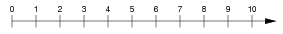
Computer simulations of causal physical processes happening over a time period are typically either clocked or event-driven. A clocked simulation quantizes time into discrete steps, typically equally spaced. Such an approach is a good way to approximate a continuous process, as long as the timestep is small enough. For instance, a clocked simulator could use a timebase of 1 millisecond (ms), and would simulate the properties of the physical system at 0 ms, 1 ms, etc:
At each multiple of the timestep, the state of the system is explicitly represented, and then used to calculate the state one time step in the future.
Clocked simulations are appropriate primarily when the physical events of interest occur at relatively uniformly distributed times. On the other hand, if the most important physical events occur at widely spaced intervals, a clocked simulator is not very efficient. A clocked simulator must either simulate many unwanted time steps between interesting events, or else use a large time step and thus have only limited detail during the interesting events.
Event-driven simulations
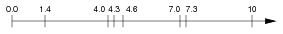
Discrete event-driven simulators have the opposite features. Such simulators explicitly model only isolated events, ignoring long periods with little of interest in between. For instance, such simulators are often used for modeling neuron membrane potentials, which change relatively slowly for long periods, but then quickly vary over a large range during a sudden firing event. An event-driven simulator can devote more timesteps to such interesting events, without spending extra time in between. For instance, such a simulator might explicitly calculate only the points listed here, skipping the times in between:
Topographica simulations
Topographica is designed to support both major types of simulations. For full generality, the underlying architecture is event driven, because it is possible to use an event-driven simulator for clocked simulations (by treating clock ticks as events), but not vice versa.
A Topographica simulation consists of:
An Event Queue:
A single globally ordered list of all events scheduled to occur in the future on the timeline; not normally accessed by a user.
EventProcessors:
Objects (typically Sheets) capable of sending and/or receiving discrete Events.
Events:
Messages that can be delivered to an EventProcessor at a specified time.
Connections:
Links between EventProcessors along which Events are passed after a (typically) fixed delay.
For instance, a typical Topographica simulation will consist of a set of Sheets connected into a graph with fixed delays:
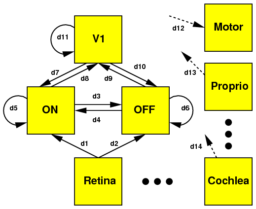
For a clocked simulation, at least one of these EventProcessors (typically an input Sheet like the Retina in this example) will generate a regular series of Events, which will cause events to be sent out over the Connections, at which point the EventProcessors will likely create new Events and send them out over their own connections, leading to a cascade of activity.
For instance, in this example, if the event queue were initally empty but the Retina generated an event at time zero, the next computation would occur at simulated time d1 or d2, when the first event arrives at the ON or OFF sheet. Subsequent events would be delivered along each of the connections, causing each Sheet to be activated in turn.
Event-driven simulations are nearly identical to this, except that instead of a regular stream of input events they will be given an irregular stream consisting of only the important events. EventProcessors will then calculate their state at each event based on the preceding events and the elapsed time. Events will still propagate as before, but not on any regular timebase.
By convention, the delays in clocked Topographica simulations are typically set up so that the user-visible state is visible on even multiples of 1.0 time. For instance, a two-Sheet simulation with a Retina and V1 might be set up to have a Connection with delay 0.5, so that the event is generated in the retina at time zero, then delivered to V1 at time 0.5, so that V1’s response will be ready for visualization by time 1.0.
To study the individual events that are generated during the simulation, you can enable verbose messaging.