Interfacing to external simulators

Topographica supports a large class of models well, but there are many models already implemented in other simulators that would take a lot of effort to reimplement. Moreover, there are many at different levels of analysis not well supported by Topographica, such as simulations that include detailed internal structure for each neuron. In order to provide a consistent framework for evaluating competing models of the same phenomena, and for integrating models at different levels, it can be useful to connect external simulators to Topographica. Such simulators include NEURON and GENESIS, focusing on detailed studies of individual neurons or very small networks of them, and NEST, focusing on large networks of simple spiking neurons.

The general problem of interfacing between simulators is quite difficult, for a variety of technical and conceptual reasons. Even so, in Topographica the process can in many cases be relatively simple, for three main reasons:

1. Many simulators now have Python interfaces, which makes it much simpler to establish the basic lines of communication between them and Topographica.
2. Even if the external simulator does not have its own Python interface, Python supports a wide variety of well-supported ways to call code written in other languages. In particular, Topographica provides very simple interface mechanisms for external C/C++ or Matlab code.
3. Perhaps most importantly, the abstractions implemented in Topographica, i.e. the Sheet interface within a general event-driven framework, provide a set of concepts shared between models formulated at very different levels, making it reasonable to compare such models and connect them within the same framework.

To be more specific, there is a very large and wide-ranging class of models that share the property of having an array of neural units whose firing rate is important for some computations. For instance, even if the underlying units are spiking, and all of their computation is based on spikes, many neurophysiological experiments are based on measuring firing rates or average activity levels. In Topographica these experiments can be formulated once, at a general level, and then applied to any model that can fit into the Topographica framework, spiking or not.

Interfacing to Topographica will be straightforward for a simulation in any language that contains a large number of neurons at any level of complexity arranged into a two-dimensional array (or a three-dimensional stack of such two-dimensional arrays). Integrating such a model into Topographica will, in turn, be useful if there are meaningful types of analysis that rely only on an average (firing rate) activation level for each neuron. Many such routines based on firing rates are implemented in a fully general form in Topographica, such as measuring receptive fields, tuning curves, and feature preference maps, decoding activity values, and 1D, 2D, or 3D activity or map plotting.

To be a part of Topographica, a model will generally need to support one or more Sheet objects. A Sheet is required to have a fixed area and density of neurons, and to be able to generate a floating-point array of the appropriate size when asked for its current pattern of activity. Once this activity matrix is available for a new Sheet type, then nearly all of Topographica’s analysis and plotting code can be used with the new Sheet type, e.g. to decode neural responses from the firing rate, or to measure a topographic map. This general-purpose interface is what makes it practical to wrap around a wide variety of external simulations, as long as they can be interpreted as a two-dimensional array that can have some average firing-rate activity value.

To demonstrate concretely the procedure for connecting external simulations to Topographica, in the following section we present a detailed example of wrapping an external NEST simulation using the Topographica Sheet interface. Shorter examples of how to interface with a variety of other simulators follow.

Interfacing to Perrinet retinal model in PyNN

For this example, we wrapped a spiking retinal ganglion cell model (examples/perrinet_retina_pynest.py) being developed by Laurent Perrinet (INCM/CNRS) as part of the FACETS project and used in a large-scale spiking model of cortical columns in V1. The external model is specified in PyNN, a Python wrapper that sets up and runs simulations of neural models relatively independently of the underlying simulation engine. This particular script calls the NEST simulator, which is well adapted for large-scale spiking neural networks, but it could also be run under NEURON by changing one line of declaration.

The model contains two populations of spiking retinal ganglion cells, a 32x32 array of ON cells and a 32x32 array of OFF cells, receiving input from a 32x32 array of photoreceptors whose activation level can be controlled externally. The code is in examples/perrinet_retina.ty, and can be run by installing PyNN, NEST, and PyNEST using Topographica’s copy of python as described in the file.

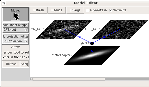
The Topographica model resulting from wrapping this network as a Photoreceptor Sheet (Photoreceptors), a connection to PyNN (PyNNR), and two ganglion cell Sheets (ON_RGC and OFF_RGC) is:

and the corresponding code is:

      import numpy
      import param
      from topo import sheet,numbergen,pattern,projection
      from topo.base.simulation import EventProcessor
(1)   import perrinet_retina_pynest as pynr

(2)   class PyNNRetina(EventProcessor):
(3)       dest_ports=["Activity"]
              src_ports=["ONActivity","OFFActivity"]
              N = param.Number(default=8,bounds=(0,None),doc="Network width")
              simtime = param.Number(default=4000*0.1,bounds=(0,None),
                  doc="Duration to simulate for each input")

              def __init__(self,**params):
                  super(PyNNRetina,self).__init__(**params)
(4)           self.ps=pynr.retina_default()
                  self.ps.update({"N":self.N})
                  self.ps.update({"simtime":self.simtime})
                  self.dt=self.ps["dt"]

(5)       def input_event(self,conn,data):
                  self.ps.update({"amplitude":.10*data})
                  on_list,off_list=pynr.run_retina(self.ps)
                  self.process_spikelist(on_list,"ONActivity")
                  self.process_spikelist(off_list,"OFFActivity")

(6)       def process_spikelist(self,spikelist,port):
                  spikes=numpy.array(spikelist)
                  spike_time=numpy.cumsum(spikes[:,0]) * self.dt
                  spike_out=pynr.spikelist2spikematrix(
                      spikes,self.N,self.simtime/self.dt,self.dt)
                  self.send_output(src_port=port,data=spike_out)

(7)   N=32
          topo.sim["PyNNR"]=PyNNRetina(N=N)

          topo.sim["Photoreceptors"]=sheet.GeneratorSheet(
               nominal_density=N, period=1.0, phase=0.05,
               input_generator=pattern.Gaussian(
                   orientation=numbergen.UniformRandom(lbound=-pi,ubound=pi,seed=1)))

          topo.sim["ON_RGC"] =sheet.ActivityCopy(nominal_density=N, precedence=0.7)
          topo.sim["OFF_RGC"]=sheet.ActivityCopy(nominal_density=N, precedence=0.7)

          topo.sim.connect("Photoreceptors","PyNNR",name=' ',
              delay=0.05,src_port="Activity",dest_port="Activity")
          topo.sim.connect("PyNNR","ON_RGC",name='  ',
              delay=0.05,src_port="ONActivity",dest_port="Activity")
          topo.sim.connect("PyNNR","OFF_RGC",name='   ',
              delay=0.05,src_port="OFFActivity",dest_port="Activity")

The example code would be nearly the same for interfacing to any other external simulation that consists of two-dimensional arrays of neurons, and so we will step through each part of this code to show how the interface is achieved. In each case, the relevant line of code is marked with a number in parentheses, which can be found on the code listing. Note that this code constitutes the complete, runnable model specification for Topographica; it is not an excerpt or summary, but is all that is required to run the external simulation within Topographica.

(1) First, the external simulation is imported, making anything available to Python from that simulation also available to Topographica. For this import to succeed, PyNN, NEST, and PyNEST need to be installed, and each need to have been given Topographica’s copy of Python during installation so that they will be available to Topographica.

(2) Next, we define a new type of Topographica EventProcessor PyNNRetina to handle communication between Topographica and the external simulator. This class simply accepts an incoming event from Topographica that contains a matrix of photoreceptor activity, passes the matrix to the external spiking simulator, collects the firing-rate-averaged results, and sends them out to any Topographica sheets that may be connected.

(3)More specifically, the class first declares that it can accept an incoming event on a port labeled Activity, and that it will generate two separate types of output data to be made available on the ONActivity and OFFActivity dest_ports. It also declares that it has two user-controlled parameters, N (size of array of neurons) and simtime (duration to run the simulation for each input). (Additional parameters from the underlying simulator can be declared similarly, or all of the underlying parameters could be exposed as a batch using suitable gluing code.)

(4) The constructor (__init__) does any initialization that should be done once per run, here consisting only of defining some parameters, but potentially including launching an external simulator, making a connection to an existing simulator, etc.

(5) The input_event method is called by Topographica whenever an Event delivers data to this object’s src_port (Activity). In this case, the method adds the incoming activity matrix into its parameters data structure (ps), and then calls the external function run_retina to run the underlying simulation. When the external simulator completes, two lists of spikes are returned, one for ON and one for OFF, and these are processed using the helper function process_spikelist. (6) For each list, process_spikelist computes the firing rate of each neuron and sends the resulting floating-point arrays out the appropriate port.

(7)The remainder of the code instantiates a model network to display the results from this class, defining one PyNNR object, a Photoreceptors Sheet to generate input patterns, two RGC Sheets to display the resulting activity patterns, and connections between them.

With this interface in place, the external simulation can be used with nearly all of Topographica’s features. For instance, the model editor image above shows one example input pattern and the resulting pattern of ON and OFF RGC activity. For this example, the main benefit to having the Topographica wrapper is to be able to present any of the types of input patterns in Topographica’s large library of input patterns, using either the GUI or systematically using Python code. For other simulations, e.g. those including cortical areas such as V1, Topographica can compute tuning curves, receptive fields, preference maps, and other types of analyses and plots for any of the neurons and Sheets available to Topographica. As long as the computation only requires average firing rates, no special-purpose code or additional interface will be needed beyond what is shown in this example. Thus Topographica can be used to provide a consistent set of analyses and plots for a wide variety of underlying simulations.

Interfacing to other Python code (e.g., PyNEST, NEURON)

The general approach outlined above can be used for any other model running in an external simulator that has a Python interface. In each case, a new Topographica EventProcessor class can be created to accept incoming events, process them somehow, and generate appropriate output. For instance, similar steps would have been used if the retina model had been written in PyNEST directly rather than PyNN, or in NEURON’s own Python interface. As long as the external simulator can be told to use Topographica’s copy of Python, then Topographica can import the required functions, execute them as part of such a class, and thus control its input and output.

Interfacing to Matlab

Topographica can also connect easily to external simulations running in Matlab, using the Python<->Matlab interface package mlabwrap that is supplied with Topographica.

For instance, the following complete, runnable Topographica script defines a small Python/numpy array x and then calls a Matlab function ``plot’’ to visualize it:

from mlabwrap import mlab
import numpy
x=numpy.array([1,2,4])
mlab.plot(x)

Any Matlab function (including user scripts) can be called similarly, with seamless interchange of scalar and array data between the two systems. This capability makes it simple to develop interfaces like the one outlined above, or just to use small bits of Matlab code when appropriate.

Interfacing to C/C++

Python offers a wide variety of methods for interfacing to C or C++ code, any of which could be used with Topographica. The specific interface currently used for the performance-critical portions of Topographica is Weave, which allows snippets of C or C++ code to be called easily from within Python code. A sample complete, runnable Topographica script with C code is:

import weave,numpy
a=numpy.array([1.0,2.0,3.0])
code = """printf("Hello, world %f\n",a[1]);"""
weave.inline(code,["a"])

Here the C printf function is being used with a Python/numpy array, and will print Hello, world 2.000000 when run. The first time it is run the C compiler will be called automatically to compile that code fragment, and then the saved object file will be reused in subsequent calls and on subsequent runs, unless the C code string is changed. This approach makes it simple to include bits of existing C code to optimize specific functions, or to make calls to C libraries.

Notes

As the examples above show, very little coding is required to wrap even complex simulations into the basic Sheet and EventProcessor components used in Topographica. A large class of models across different modelling and analysis levels (e.g., firing-rate, integrate-and-fire, and compartmental neuron models) can fit into this structure, allowing all of them to be analyzed and compared consistently, interconnected where appropriate, and explored visually even if the underlying simulator has no graphical interface (as for NEST). Although the general problem of simulator interoperatibility is difficult to address, in this specific case it is relatively easy to get practical benefits from combining simulators.

While the approach outlined above is general purpose, it does require coding a Topographica component to match each specific model implemented externally. A useful but more complex alternative would be to provide a detailed mapping between object types in an external simulator. For instance, one could provide a Topographica Sheet object that instantiates a corresponding NEST layer object, and similarly for a Topographica Projection object and a NEST connection object. In this way NEST or other simulators could be used to provide specific functionality missing from Topographica, rather than to implement complete models. However, developing such interfaces is much more involved than the simple wrapping described here.

Even though the Topographica Sheet interface is general enough to fit a wide range of current models, there are some models that do not fit within its assumptions. In particular, a Sheet needs to have an underlying grid shape to the population of neurons, though individual neurons can be at jittered spatial locations (or sometimes absent), as long as no more than one neuron is present in any grid cell. Also, only Cartesian grids are currently supported; hexagonal grids could be added in the future. Arbitrary 3D locations will be difficult to support except by imposing a 3D grid. Note that nonlinear spacings are supported, using arbitrary coordinate mapping between Sheets, e.g. for foveated retinotopic mappings, as long as there is still an underlying grid of neurons.

In summary, working at the topographic map level makes it practical to provide interconnections between models and simulators working at different levels of detail. As long as the neurons are grouped into two-dimensional sheets of related units, they will be able to interface easily with Topographica’s tools and components. The result provides a shared platform for evaluating models from different sources, allowing consistent analysis and testing even for very different implementations.