LISSOM Orientation Map

This tutorial shows how to use the Topographica software package to explore a simple orientation map simulation using test patterns and weight plots. This particular example uses a LISSOM model cortex, which has been used extensively in publications (e.g. Miikkulainen et al., 2005) but is no longer recommended for new work, because it has been superseded by the simpler but more robust GCAL model. Although we focus on one model in this tutorial, Topographica provides support for many other models and allows a very large family of models to be constructed from the same components.

This tutorial assumes that you have already followed the instructions for obtaining and installing Topographica. Also, you will need to generate a saved orientation map network (a .typ file), which can be done from a Unix or Mac terminal or Windows command prompt by running

topographica -a -c "generate_example('lissom_oo_or_10000.typ')"

Depending on the speed of your machine, you may want to go get a snack at this point; on a 3GHz 512MB machine this training process currently takes from 7-15 minutes (depending on the amount of level 2 cache). When training completes, lissom_oo_or_10000.typ will be saved in Topographica’s output path ready for use in the tutorial.

Response of an orientation map

In this example, we will load a saved network and test its behavior by presenting different visual input patterns.

1. First, start the Topographica GUI from a terminal:

   topographica -g
   

   (Windows users can instead double click on the desktop Topographica icon.) This will open the Topographica console:

   

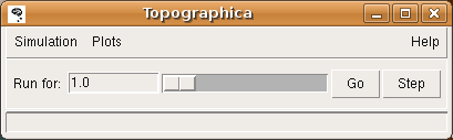
   The window and button style will differ on different platforms, but similar buttons should be provided.

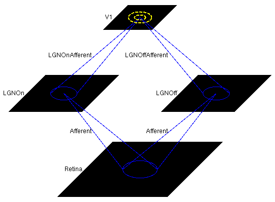
2. Next, load the saved network by selecting selecting Load snapshot from the Simulation menu and selecting lissom_oo_or_10000.typ. This small orientation map simulation should load in a few seconds, with a 54x54 retina, a 36x36 LGN (composed of one 36x36 OFF channel sheet, and one 36x36 ON channel sheet), and a 48x48 V1 with about two million synaptic weights. The architecture can be viewed in the Model Editor window (which can be selected from the Simulation menu), but is also shown below:

   

3. To see how this network responds to a simple visual image, first open an Activity window from the Plots menu on the Topographica Console, then select Test pattern from the Simulation menu to get the Test Pattern window:

   

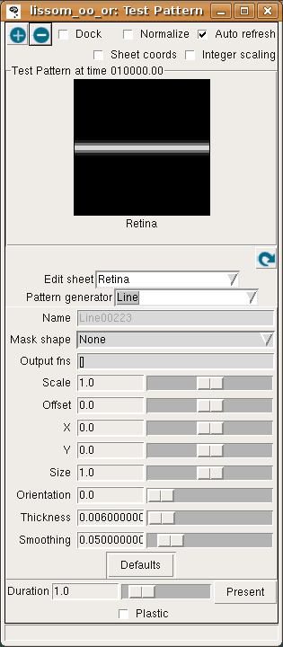
   Then select a Line Pattern generator, and hit Present to present a horizontal line to the network.

4. The Activity window should then show the result:

   

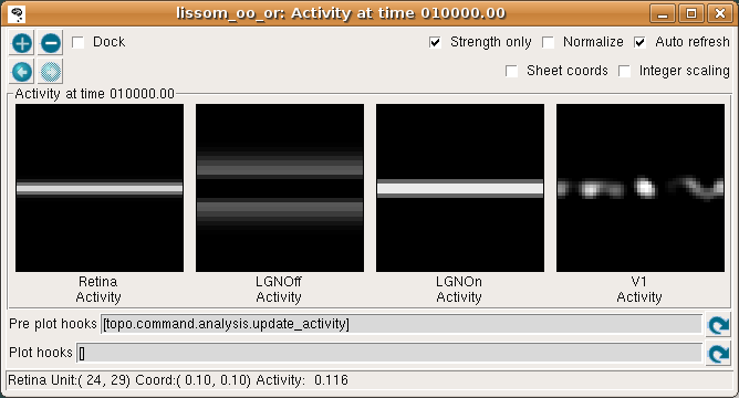
   This window shows the response for each neural area. For now, please turn on Strength only; it is usually off by default.

   As you move your mouse over the plots, information about the location of the mouse cursor is displayed in the status bar at the bottom of the window. For these plots, you can see the matrix coordinates (labeled “Unit”), sheet coordinates (labeled “Coord”), and the activity level of the unit currently under the pointer.

   In the Retina plot, each photoreceptor is represented as a pixel whose shade of gray codes the response level, increasing from black to white. This pattern is what was specified in the Test Pattern window. Similarly, locations in the LGN that have an OFF or ON cell response to this pattern are shown in the LGNOff and LGNOn plots. At this stage the response level in V1 is also coded in shades of gray, and the numeric values can be found using the pointer.

   From these plots, you can see that the single line presented on the retina is edge-detected in the LGN, with ON LGN cells responding to areas brighter than their surround, and OFF LGN cells responding to areas darker than their surround. In V1, the response is patchy, as explained below.

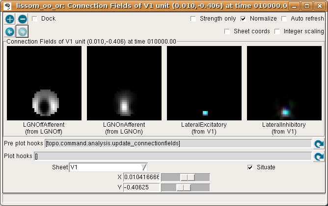
5. To help understand the response patterns in V1, we can look at the weights to V1 neurons. These weights were learned previously, as a result of presenting 10000 pairs of oriented Gaussian patterns at random angles and positions. To plot a single neuron, select Connection Fields from the Plots menu. This will plot the synaptic strengths of connections to the neuron in the center of the cortex (by default):

   

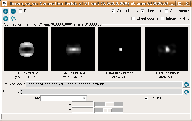
   Again, for now please turn on Strength only; it is usually off by default.

   The plot shows the afferent weights to V1 (i.e., connections from the ON and OFF channels of the LGN), followed by the lateral excitatory and lateral inhibitory weights to that neuron from nearby neurons in V1. The afferent weights represent the retinal pattern that would most excite the neuron. For the particular neuron shown above, the optimal retinal stimulus would be a short, bright line oriented at about 0 degrees (from 9 o’clock to 3 o’clock) in the center of the retina. (Note that the particular neuron you are viewing may have a different preferred orientation.)

6. If all neurons had the same weight pattern, the response would not be patchy – it would just be a blurred version of the input (for inputs matching the weight pattern), or blank (for other inputs). To see what the other neurons look like, select Projection from the Plots menu, then select LGNOnAfferent from the drop-down Projection list, followed by the refresh arrow next to ‘Pre plot hooks’:

   

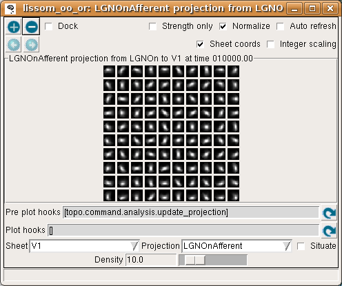
   This plot shows the afferent weights from the LGN ON sheet for every fifth neuron in each direction. You can see that most of the neurons are selective for orientation (not just a circular spot), and each has a slightly different preferred orientation. This suggests an explanation for why the response is patchy: neurons preferring orientations other than the one present on the retina do not respond. You can also look at the LateralInhibitory weights instead of LGNOnAfferent; those are patchy as well because the typical activity patterns are patchy.

7. To visualize all the neurons at once in experimental animals, optical imaging experiments measure responses to a variety of patterns and record the one most effective at stimulating each neuron. The results of a similar procedure can be viewed by selecting Plots > Preference Maps > Orientation Preference:

   

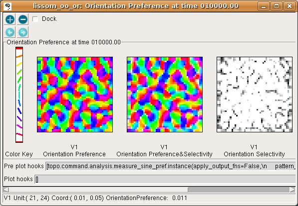
   The Orientation Preference plot is the orientation map for V1 in this model. Each neuron in the plot is color coded by its preferred orientation, according to the key shown to the left of the plot. (If viewing a monochrome printout, see web page for the colors). Note that phase preference and selectivity are also displayed in the window, but these are not analyzed here (and are not shown above).

   You can see that nearby neurons have similar orientation preferences, as found in primate visual cortex. The Orientation Selectivity plot shows the relative selectivity of each neuron for orientation on an arbitrary scale; you can see that in this simulation nearly all neurons became orientation selective. The Orientation Preference&Selectivity plot shows the two other Orientation plots combined – each neuron is colored with its preferred orientation, and the stronger the selectivity, the brighter the color. In this case, because the neurons are strongly selective, the Preference&Selectivity plot is nearly identical to the Preference plot.

   If you want to see what happens during map measurement, you can watch the procedure as it takes place by enabling visualization. Edit the ‘Pre plot hooks’ (as described in the Changing existing plots section of the User Manual) so that the measure_sine_pref command’s display parameter is turned on. Open an Activity window and ensure it has Auto-Refresh turned on, then press Refresh by the Orientation Preference window’s ‘Pre plot hooks’. You will see a series of sine gratings presented to the network, and can observe the response each time in the LGN and V1 sheets. When you are done, press Refresh on the pre-plot hooks in the Activity window to restore the original activity pattern plots.

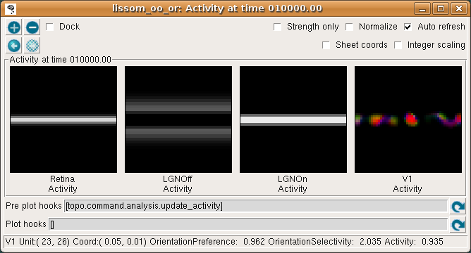
8. Now that we have looked at the orientation map, we can see more clearly why activation patterns are patchy by coloring each neuron with its orientation preference. To do this, make sure that Strength only is now turned off in the Activity window:

   

   

   Each V1 neuron is now color coded by its orientation, with brighter colors indicating stronger activation. Additionally, the status bar beneath the plots now also shows the values of the separate channels comprising the plot: OrientationPreference (color), OrientationSelectivity (saturation), and Activity (brightness).

   The color coding allows us to see that the neurons responding are indeed those that prefer orientations similar to the input pattern, and that the response is patchy because other nearby neurons do not respond. To be sure of that, try selecting a line with a different orientation, and hit present again – the colors should be different, and should match the orientation chosen.

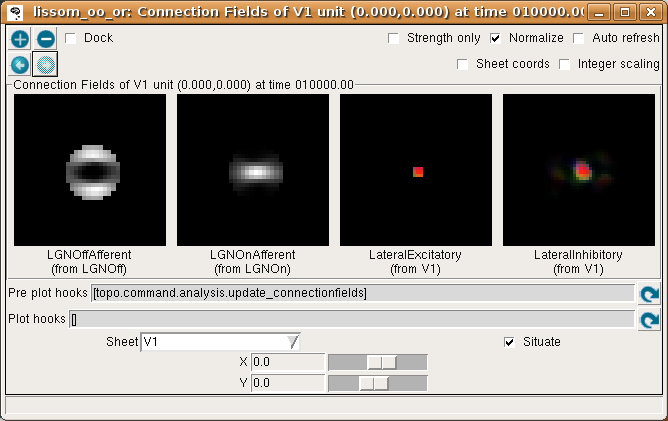
9. If you now turn off Strength only in the Connection Fields window, you can see that the neuron whose weights we plotted is located in a patch of neurons with similar orientation preferences:

   

   

   Look at the LateralExcitatory weights, which show that the neurons near the above neuron are nearly all red, to match its preferred orientation.

   Returning to the Test pattern window, try presenting a vertical line (orientation of pi/2) and then, in the Activity window, right click on one of the cyan-colored patches of activity. This will bring up a menu:

   

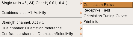
   The menu offers operations on different parts of the plot: the first submenu shows operations available on the single selected unit, and the second shows operations available on the combined (visible) plot. The final three submenus show operations available on each of the separate channels that comprise the plot.

   Here we are interested to see the connection fields of the unit we selected, so we choose Connection Fields from the Single unit submenu to get a new plot:

   

   

   This time we can see from the LateralExcitatory weights that the neurons near this one are all colored cyan (i.e., are selective for vertical).

10. Right-click menus are available on most plots, and provide a convenient method of further investigating and understanding the plots. For instance, on the Orientation Preference window, the connection fields of units at any location can easily be visualized, allowing one to see the connection fields of units around different features of the map.

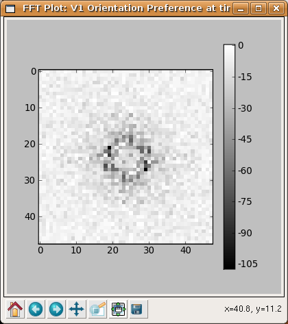
    As another example, an interesting property of orientation maps measured in animals is that their Fourier spectrums usually show a ring shape, because the orientations repeat at a constant spatial frequency in all directions. Selecting Hue channel: OrientationPreference > Fourier transform from the right-click menu allows us to see the same is true of the map generated by the LISSOM network:

    

11. Now that you have a feel for the various plots, you can try different input patterns, seeing how the cortex responds to each one. Just select a Pattern generator, e.g. Gaussian, Disk, or SineGrating, and then hit Present.

    For each Pattern generator, you can change various parameters that control its size, location, etc.:

    orientation

    controls the angle (try pi/4 or -pi/4)

    x and y

    control the position on the retina (try 0 or 0.5)

    size

    controls the overall size of e.g. Gaussians and rings

    aspect_ratio

    controls the ratio between width and height; will be scaled by the size in both directions

    smoothing

    controls the amount of Gaussian falloff around the edges of patterns such as rings and lines

    scale

    controls the brightness (try 1.0 for a sine grating). Note that this relatively simple model is very sensitive to the scale, and scales higher than about 1.2 will result in a broad, orientation-unselective response, while low scales will give no response. More complex models (and actual brains!) are less sensitive to the scale or contrast.

    offset

    is added to every pixel

    frequency

    controls frequency of a sine grating or Gabor

    phase

    controls phase of a sine grating or Gabor

    mask_shape

    allows the pattern to be masked by another pattern (e.g. try a mask_shape of Disk or Ring with a SineGrating or UniformRandom pattern). The parameters of the mask_shape pattern can be edited by right-clicking on it.

    To present photographs, select a Pattern generator of type FileImage. (You can type the path to an image file of your own (in e.g. PNG, JPG, TIFF, or PGM format) in the filename box.) For most photographs you will need to change the scale to something like 2.0 to see a reasonable response from this model V1, and you may want to enlarge the image size to look at details. A much larger, more complicated, and slower map would be required to see interesting patterns in the response to most images, but even with this network you may be able to see some orientation-specific responses to large contours in the image:

    

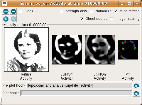
    Here we have enabled Sheet coords so that each plot will be at the correct size relative to each other. That way, the location of a given feature can be compared between images. In this particular network, the Retina and LGN stages each have an extra “buffer” region around the outside so that no V1 neuron will have its CF cut off, and the result is that V1 sees only the central region of the image in the LGN, and the LGN sees only the central region of the retina. (Sheet coordinates are normally turned off because they make the cortical plots smaller, but they can be very helpful for understanding how the sheets relate to each other.)

12. The procedure above allows you to explore the relationship between the input and the final response after the cortex has settled due to the lateral connections. If you want to understand the settling process itself, you can also visualize how the activity propagates from the retina to the LGN, from the LGN to V1, and then within V1. To do this, first make sure that there is an Activity window open, with Auto-refresh enabled. Then go to the console window and hit “Step” repeatedly. After an input is presented, you will see the activity arrive first in the LGN, then in V1, and then gradually change within V1. The Step button moves to the next scheduled event in the simulation, which are at even multiples of 0.05 for this particular simulation. You can also type in the specific duration (e.g. 0.05) to move forward into the “Run for:” box, and hit “Go” instead.

    As explained in the User Manual, this process is controlled by the network structure and the delays between nodes. For simplicity, let’s consider time starting at zero. The first scheduled event is that the Retina will be asked to draw an input pattern at time 0.05 (the phase of the GeneratorSheet). Thus the first visible activity occurs in the Retina, at 0.05. The Retina is connected to the LGN with a delay of 0.05, and so the LGN responds at 0.10. The delay from the LGN to V1 is also 0.05, so V1 is first activated at time 0.15. V1 also has self connections with a delay of 0.05, and so V1 is then repeatedly activated every 0.05 timesteps. Eventually, the number of V1 activations reaches a fixed limit for LISSOM (usually about 10 timesteps), and no further events are generated or consumed until the next input is generated at time 1.05. Thus the default stepsize of 1.0 lets the user see the results after each input pattern has been presented and the cortex has come to a steady state, but results can also be examined at a finer timescale. Be sure to leave the time clock at an even multiple of 1.0 before you do anything else, so that the network will be in a well-defined state. (To do this, just type the fractional part into the “Run for:” box, i.e. 0.95 if the time is currently 10002.05, press “Go”, and then change “Run for:” to 1.0.)

Learning (optional)

The previous examples all used a network trained previously, without any plasticity enabled. Many researchers are interested in the processes of development and plasticity. These processes can be studied using the LISSOM model in Topographica as follows.

1. First, quit from any existing simulation, and get a copy of the example files to work with if you do not have them already. Then start a new run of Topographica:

   topographica -g
   

   From the Simulation menu, select Run Script. Then from the models directory, open lissom_oo_or.ty.

2. Next, open an Activity window and make sure that it has Auto-refresh enabled. Unless your machine is very slow, also enable Auto-refresh in a Projection window showing LGNOnAfferent. On a very fast machine you could even Auto-refresh an Orientation Preference window (probably practical only if you reduce the nominal_density of V1).

3. Now hit Go a few times on the Topographica Console window, each time looking at the random input(s) and the response to them in the Activity window. The effect on the network weights of learning this input can be seen in the Projection window.

4. With each new input, you may be able to see small changes in the weights of a few neurons in the LGNOnAfferent array (by peering closely). If the changes are too subtle for your taste, you can make each input have an obvious effect by speeding up learning to a highly implausible level. To do this, open the Model Editor window, right click on the LGNOnAfferent projection (the cone-shaped lines from LGNOn to V1), select Properties, and change Learning Rate from the default 0.48 to 100, press Apply, and then do the same for the LGNOffAfferent projection. Now each new pattern generated in a training iteration will nearly wipe out any existing weights.

5. For more control over the training inputs, open the Test Pattern window, select a Pattern generator, e.g. Disk, and other parameters as desired. Then enable Plastic in that window, and hit Present. You should again see how this input changes the weights, and can experiment with different inputs.

6. Once you have a particular input pattern designed, you can see how that pattern would affect the cortex over many iterations. To do so, open a Model Editor window and right click on the Retina’s diagram, then select Properties from the resulting menu. In the Parameters of Retina window that opens, select the pattern type you want to use for the Input Generator item, and then right click on that pattern, choose Properties and, in the new window, modify any of its parameters as you wish. Note that you will probably want to have dynamic values for certain parameters. For instance, to have a random orientation for each presentation, right click on Orientation and select Enter dynamic value. The slider will disappear from the entry box, and you can type in an expression such as numbergen.UniformRandom(lbound=-pi,ubound=pi). When you have finished configuring your pattern, press Apply or Close on the Parameters of Gaussian window. Having now set up the input generator on the Parameters of Retina window, click Apply or Close on this too. Now when you press Go on the console window (assuming Run for is set to 1), you should see your pattern being presented in the Activity Window.

7. After a few steps (or to do e.g. 20 steps in a row, change Run for to 20 and press return) you can plot (or refresh) an Orientation Preference map to see what sort of orientation map has developed. (Press the ‘Refresh’ button next to the Pre plot hooks if no plot is visible when first opening the window. Measuring a new map will usually take about 15 seconds to complete.) If you’ve changed the learning rate to a high value, or haven’t presented many inputs, the map will not resemble actual animal maps, but it should still have patches selective for each orientation.

8. If you are patient, you can even run a full, more realistic, simulation with your favorite type of input. To do this, quit and start again, then change the Retina’s Input generator as before via the Model Editor, but make sure not to change the learning rate this time. Then you can change Run for to 10000 and press Go to see how a full simulation would work with your new inputs. Running for 10000 iterations will likely take at least several minutes for recent machines; if you are less patient, try doing 1000 iterations at a time instead before looking at an Orientation Preference map.

9. If you are really patient, you can change the number of units to something closer to real primate cortex, by quitting and then restarting with a higher density in V1. To do this, you will need to specify the example script from the commandline. The path of the lissom_oo_or.ty script was printed by Topographica in step 1 of this Learning section, but if you are not sure where the examples are located, you can find out by first running

   topographica -c "from topo.misc.genexamples import print_examples_dir; print_examples_dir()"
   

   Then you can use the path to the example, as well as specifying a higher cortex density, e.g.

   topographica -p cortex_density=142 ~/Documents/Topographica/examples/lissom_oo_or.ty -g
   

   You’ll need about a gigabyte of memory and a lot of time, but you can then step through the simulation as above. The final result after 10000 iterations (requiring several hours on a 3GHz machine) should be a much smoother map and neurons that are more orientation selective. Even so, the overall organization and function should be similar.

Exploring further

To see how the example works, load the lissom_oo_or.ty file into a text editor and see how it has been defined, then find the corresponding Python code for each module and see how that has been defined.

Topographica comes with additional examples, and more are always being added. In particular, the above examples work in nearly the same way with the simpler lissom_or.ty model that has no LGN. Any valid Python code can be used to control and extend Topographica; documentation for Python and existing Topographica commands can be accessed from the Help menu of the Topographica Console window.

Please contact jbednar@inf.ed.ac.uk if you have questions or suggestions about the software or this tutorial.